Recurrent Neural Networks
Introduction
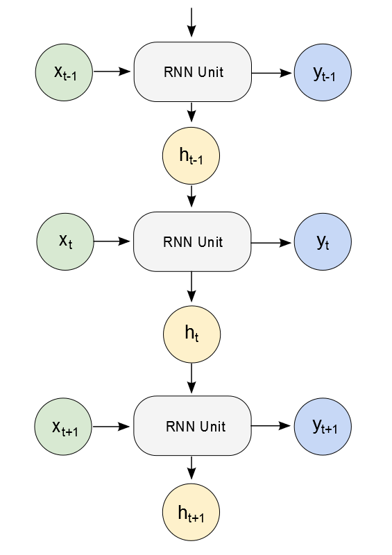
Recurrent Neural Network (RNN) is a neural network which has at least one feedback loop. RNN defines a non-linear dynamic system which can learn the mapping from input sequences to output sequences. RNN is considered the deepest of all neural networks. RNN has many forms and the simplest one is a Multilayer Perceptron where previous hidden nodes feed back into the network.

Figure 1: Recurrent Neural Network
For language modeling (i.e. predicting the next word based on previous words), RNN significantly outperforms the standard N-gram-based methods.
However, RNN is difficult to train since it suffers from the vanishing / exploding gradient effects where error signals become smaller and smaller (in the vanishing case) / larger and larger (in the exploding case) when back-propagating errors from output layer back to input layer.

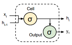
Figure 2: RNN Unit (adapted from [1])
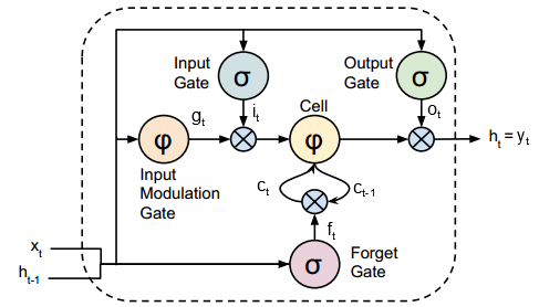
Long Short-Term Memory (LSTM) is a variant of RNN which was proposed to resolve the vanishing / exploding gradient problems. LSTM has memory nodes that helps the network learn when to forget previous hidden states and when to update hidden states given new input. LSTM has been used very successfully in handwriting recognition.

Figure 3: LSTM Unit (adapted from [1])
where \(\sigma\) is sigmoid function, \(\varphi\) is tanh function, and \(\odot\) is element-wise product.
Backpropagation
An RNN with the length \(T\) is actually a feed-forward neutral network with the depth \(T\). For simplicity, here we will derive backpropagation steps to train the vanilla RNN (Figure 2) for a classification task.
Given a training data set \(D = \{(X_i, \bar{Y}_i)\}_{i=1}^N\), where \(X_i\) and \(\bar{Y}_i\) are two sequences with length \(T\), \(X_i=(X_{i1}, ..., X_{iT})\), \(\bar{Y}_i=(\bar{Y}_{i1}, ..., \bar{Y}_{iT})\), the loss function is a log-loss, i.e. cross entropy between the ground truth sequence \(\bar{Y}\) and the predicted sequence \(Y\):
\[L(\bar{Y}, Y) = \frac{1}{N}\sum_{i=1}^N \frac{1}{T} \sum_{t=1}^T CE(\bar{Y}_{it}, Y_{it})\]where \(CE(\bar{y}, y) = -\sum_{l=1}^L \bar{y}^l \log y^l\) (\(L\) is the number of labels, \(\bar{y}^l\) and \(y^l\) are components of the vectors \(\bar{y}\) and \(y\) respectively).
Stochastic Gradient Descent (SGD) will be used for training. Assuming one training example is provided at a time, the loss function becomes \(L(\bar{Y}, Y) = \frac{1}{T} \sum_{t=1}^T CE(\bar{y}_t, y_t)\).
\(L(\bar{Y}, Y)\) minimizes \(\Longleftrightarrow\) \(\sum_{t=1}^T CE(\bar{y}_t, y_t)\) minimizes.
The forward pass is pretty straightforward as shown in Figure 2. The backward pass is quite tricky due to the link between \(h_{t-1}\) and \(h_t\).
We will backpropagate the error from \(t = T\) back to \(t = 1\):
1) Backpropagate to \(y_t^{raw} = W_{hy} h_t + b_y\)
Assuming that the ground truth label is \(l\), we have
\[L_t = CE(\bar{y}_t, y_t) = - \log y_l = - y_l^{raw} + \log A\]where \(y = softmax(y^{raw})\) and \(A\) is \(softmax\)’s normalization factor.
\[\frac{\partial L_t}{\partial y_t^{raw}} = -1 + \frac{1}{A} \times \frac{\partial A}{\partial y_t^{raw}} = -1 + \frac{1}{A} \times A \times e^{y_t^{raw}} = -1 + e^{y_t^{raw}}\]2) Backpropagate to \(W_{hy}\) and \(b_y\)
\[\begin{align} \frac{\partial L_t}{\partial W_{hy}} &= \frac{\partial L_t}{\partial y_t^{raw}} \times \frac{\partial y_t^{raw}}{\partial W_{hy}} = \frac{\partial L_t}{\partial y_t^{raw}} \times h_t \\ \frac{\partial L_t}{\partial b_y} &= \frac{\partial L_t}{\partial y_t^{raw}} \end{align}\]3) Backpropagate to \(h_t^{raw}\)
\[\frac{\partial L_t}{\partial h_t^{raw}} = \frac{\partial L_t}{\partial h_t} \times \frac{\partial h_t}{\partial h_t^{raw}} = \frac{\partial L_t}{\partial h_t} \times h_t \times (h_t - 1)\]since \(h_t = \sigma(h_t^{raw})\).
4) Backpropagate to \(h_t\)
Since both \(L_t\) and \(L_{t+1}\) depend on \(h_t\), we need to consider both of them for this backpropagation step:
\[\begin{align} \frac{\partial (L_t + L_{t+1})}{\partial h_t} &= \frac{\partial L_t}{\partial h_t} + \frac{\partial L_{t+1}}{\partial h_t} \\ &= \frac{\partial L_t}{\partial y_t^{raw}} \times \frac{\partial y_t^{raw}}{\partial h_t} + \frac{\partial L_{t+1}}{\partial h_{t+1}^{raw}} \times \frac{\partial h_{t+1}^{raw}}{\partial h_t} \\ &= \frac{\partial L_t}{\partial y_t^{raw}} \times W_{hy} + \frac{\partial L_{t+1}}{\partial h_{t+1}^{raw}} \times W_{hh} \\ \end{align}\]5) Backpropagate to \(W_{xh}\), \(W_{hh}\), and \(b_h\)
\[\begin{align} \frac{\partial L_t}{\partial W_{xh}} &= \frac{\partial L_t}{\partial h_t^{raw}} \times x_t \\ \frac{\partial L_t}{\partial W_{hh}} &= \frac{\partial L_t}{\partial h_t^{raw}} \times h_{t-1} \\ \frac{\partial L_t}{\partial b_h} &= \frac{\partial L_t}{\partial h_t^{raw}} \end{align}\]Implementation
For the implementation, we will try out a basic RNN model which learns Python syntax. Character sequences from the source code are fed into the training and label sequences \(X_i\) and \(\bar{Y}_i\) where each character \(X_{it}\) is used to predict its next character \(Y_{it}\).
Unlike the previous post which uses Theano, we will use Google’s TensorFlow to implement the RNN model. Similar to Theano, TensorFlow provides automatic gradient calculation and even better it provides several builtin optimizer such as Adam used in the code.
Here we don’t use TensorFlow’s builtin RNN cells. However, the code to build RNN is quite easy to follow and it’s just a straightforward translation from the formula in Figure 2.
References
[1] Jeff Donahue et al. Long-term Recurrent Convolutional Networks for Visual Recognition and Description (URL).